5.2. Creating OHLC charts with Quasar#
In finance, order book data is captured for a variety of purposes. In this guide we will walk to one specific common use case for finance, converting raw order / trade data into OHLC charts.
The guide will cover:
Modeling order and trade data with Quasar;
Using Quasar’s query language to convert raw orderbook data to OHLC in real-time;
Using the Quasar Pandas API for ingestion and querying.
Completing this guide will take 30-60 minutes.
5.2.1. Preparation#
If you wish to run this guide locally, there are two ways to prepare your local development environment:
5.2.1.1. Docker#
We have prepared a pre-loaded Docker image which contains everything needed to run practice guide. To get started, please launch the bureau14/howto-ohlc-crypto Docker container as follows:
$ docker run -ti --net host bureau14/howto-ohlc-crypto:3.13.1
Launching QuasarDB in background..
Launching Jupyter lab...
[I 13:20:59.346 NotebookApp] Writing notebook server cookie secret to /home/qdb/.local/share/jupyter/runtime/notebook_cookie_secret
[I 13:20:59.501 NotebookApp] Serving notebooks from local directory: /work/notebook
[I 13:20:59.501 NotebookApp] Jupyter Notebook 6.4.6 is running at:
[I 13:20:59.501 NotebookApp] http://localhost:8888/?token=...
[I 13:20:59.501 NotebookApp]  or http://127.0.0.1:8888/?token=...
You can now navigate with your browser to the URL provided by the Jupyter notebook and continue with this exercise.
5.2.1.2. Standalone installation#
5.2.1.2.1. Install and launch QuasarDB#
Please install & launch QuasarDB for your environment; the free community edition is sufficient.
For more information and instructions on how to install QuasarDB, please follow our installation guide .
5.2.1.2.2. Download this Jupyter notebook#
You can download this notebook prepackaged from this location:
Please download this, and extract it in a folder on your local machine.
5.2.1.2.3. Prepare Python environment#
Assuming you have downloaded and extracted the Jupyter notebook, please install your environment as follows:
# Install requirements

$ python3 -m pip install -r requirements.txt

# Launch local notebook

$ jupyter notebook ./crypto-ohlc.ipynb

[I 17:16:02.496 NotebookApp] Serving notebooks from local directory: /home/user/qdb-guides/
[I 17:16:02.496 NotebookApp] Jupyter Notebook 6.4.6 is running at:
[I 17:16:02.496 NotebookApp] http://localhost:8888/?token=...
[I 17:16:02.496 NotebookApp]  or http://127.0.0.1:8888/?token=...
[I 17:16:02.496 NotebookApp] Use Control-C to stop this server and shut down all kernels (twice to skip confirmation).
A new jupyter notebook should automatically open, otherwise please manually navigate and you can navigate your browser to http://localhost:8888/ with the environment prepared.
You are now completed with the preparations.
5.2.2. Open-High-Low-Close#
In this tutorial, we will be working with raw orderbook market data: for each mutation to the orderbook, we receive and store a new record in the database.
Example mutations that can occur:
A new order is submitted to the exchange;
A trade is made between two parties;
An order is cancelled.
The volume of this data is typically huge. In order to make analysis and visualization of this data more feasible, this raw data is often converted into an Open-High-Low-Close (OHLC) shape.
According to the Wikipedia page about OHLC charts :
An open-high-low-close chart (also OHLC) is a type of chart typically used to illustrate movements in the price of a financial instrument over time. Each vertical line on the chart shows the price range (the highest and lowest prices) over one unit of time, e.g., one day or one hour.
Tick marks project from each side of the line indicating the opening price (e.g., for a daily bar chart this would be the starting price for that day) on the left, and the closing price for that time period on the right.
For us, this means we want to take the raw market data and process each symbol as follows:
Aggregate the market data into regular intervals, e.g. 1 minute;
For each interval, aggregate each of the OHLC dimensions.
In this guide you will learn how to ingest, model, and query this data.
5.2.3. Imports and setups#
Now that we have explained what OHLC data is, we can start working on the actual solution.
First let’s go through some boilerplate to import libraries and establish a connection with the QuasarDB cluster.
import datetime
import json
import random
import pprint
import copy
from tqdm import tqdm

import requests
import numpy as np
import pandas as pd
import quasardb
import quasardb.pandas as qdbpd

# Utilities for plotting waveforms
from utils import plot_stock, plot_ohlc
pp = pprint.PrettyPrinter(indent=2, sort_dicts=False)

def get_conn():
    return quasardb.Cluster("qdb://127.0.0.1:2836")

# This connection will be used for the remainder of the notebook
conn = get_conn()
5.2.4. Load sample data#
For this demo, we will pull live data from the public Coinbase API. We will be focusing on trade data only, but the same concepts apply to order data as well.
# Pull live trade data from Coinbase
def pull_data(product, max_pages=25):
    after = None

    for i in tqdm(range(max_pages)):
        if after is None:
            url = 'https://api.pro.coinbase.com/products/{}/trades'.format(product)
        else:
            url = 'https://api.pro.coinbase.com/products/{}/trades?after={}'.format(product, after)

        r = requests.get(url, timeout=15)
        results = r.json()
        for result in results:
            yield result

        if not r.headers.get('cb-after'):
            break
        else:
            after = r.headers['cb-after']

product = 'BTC-USD'
df = pd.DataFrame(pull_data(product, max_pages=100)) # decrease max_pages to pull less data
df
100%|██████████████████████████████| 100/100 [00:32<00:00, 3.09it/s]
time |
trade_id |
price |
size |
side |
|
|---|---|---|---|---|---|
0 |
2022-01-10T16:13:05.32308Z |
261952992 |
41151.00000000 |
0.01214698 |
sell |
1 |
2022-01-10T16:13:05.273736Z |
261952991 |
41151.00000000 |
0.00116054 |
sell |
2 |
2022-01-10T16:13:05.257686Z |
261952990 |
41151.00000000 |
0.00992776 |
sell |
3 |
2022-01-10T16:13:05.257686Z |
261952989 |
41150.90000000 |
0.00100000 |
sell |
4 |
2022-01-10T16:13:05.257686Z |
261952988 |
41150.08000000 |
0.00100000 |
sell |
… |
… |
… |
… |
… |
… |
99995 |
2022-01-10T14:18:52.928663Z |
261852997 |
40000.00000000 |
0.00995025 |
buy |
99996 |
2022-01-10T14:18:52.928663Z |
261852996 |
40000.00000000 |
0.00237249 |
buy |
99997 |
2022-01-10T14:18:52.928663Z |
261852995 |
40000.00000000 |
0.00125000 |
buy |
99998 |
2022-01-10T14:18:52.928663Z |
261852994 |
40000.00000000 |
0.01617267 |
buy |
99999 |
2022-01-10T14:18:52.928663Z |
261852993 |
40000.00000000 |
0.10000000 |
buy |
5.2.5. Ingesting into Quasar#
We can now ingest this data into Quasar. We can make use of the QuasarDB Pandas integration to easily store the dataframe as a table inside the database.
To do this, we need to perform the following steps:
Ensure that each trade timestamp is the dataframe’s index;
Ensure that each timestamp is a nanosecond precision datetime64;
Create a new table for this product’s trades, which we will name
products/btcusd/trades.Load the data into the table.
# Ensure our timestamps are of type datetime64[ns]
df['time'] = pd.to_datetime(df['time'])

# Price and size as well
df = df.astype({'price': 'float64',
                'size': 'float64'})


# Update our dataframe index
df = df.set_index('time', drop=True)
df
time |
trade_id |
price |
size |
side |
|---|---|---|---|---|
2022-01-10 16:13:05.323080+00:00 |
261952992 |
41151.00 |
0.012147 |
sell |
2022-01-10 16:13:05.273736+00:00 |
261952991 |
41151.00 |
0.001161 |
sell |
2022-01-10 16:13:05.257686+00:00 |
261952990 |
41151.00 |
0.009928 |
sell |
2022-01-10 16:13:05.257686+00:00 |
261952989 |
41150.90 |
0.001000 |
sell |
2022-01-10 16:13:05.257686+00:00 |
261952988 |
41150.08 |
0.001000 |
sell |
… |
… |
… |
… |
… |
2022-01-10 14:18:52.928663+00:00 |
261852997 |
40000.00 |
0.009950 |
buy |
2022-01-10 14:18:52.928663+00:00 |
261852996 |
40000.00 |
0.002372 |
buy |
2022-01-10 14:18:52.928663+00:00 |
261852995 |
40000.00 |
0.001250 |
buy |
2022-01-10 14:18:52.928663+00:00 |
261852994 |
40000.00 |
0.016173 |
buy |
2022-01-10 14:18:52.928663+00:00 |
261852993 |
40000.00 |
0.100000 |
buy |
# We can now use the QuasarDB pandas interface to create the table and store the data.
#
# To ensure we don't insert the same data multiple times, let's first drop the table if
# it already existed.
table = conn.table('products/btcusd/trades')

try:
    table.remove()
    print("removed table {}".format(table))
except:
    # Table did not yet exist
    pass

# By setting create=True, we explicitly tell the Pandas API to create the table if
# it did not yet exist.
qdbpd.write_dataframe(df, conn, table, create=True)

print("inserted dataframe")
inserted dataframe
# We can now use the same pandas API to read back the data
qdbpd.read_dataframe(table)
trade_id |
price |
size |
side |
|
|---|---|---|---|---|
2022-01-10 14:18:52.928663 |
261855692 |
40000.00 |
0.118255 |
buy |
2022-01-10 14:18:52.928663 |
261855691 |
40000.00 |
0.046940 |
buy |
2022-01-10 14:18:52.928663 |
261855690 |
40000.00 |
0.464255 |
buy |
2022-01-10 14:18:52.928663 |
261855689 |
40000.00 |
0.002500 |
buy |
2022-01-10 14:18:52.928663 |
261855688 |
40000.00 |
0.009900 |
buy |
… |
… |
… |
… |
… |
2022-01-10 16:13:05.257686 |
261952990 |
41151.00 |
0.009928 |
sell |
2022-01-10 16:13:05.257686 |
261952989 |
41150.90 |
0.001000 |
sell |
2022-01-10 16:13:05.257686 |
261952988 |
41150.08 |
0.001000 |
sell |
2022-01-10 16:13:05.273736 |
261952991 |
41151.00 |
0.001161 |
sell |
2022-01-10 16:13:05.323080 |
261952992 |
41151.00 |
0.012147 |
sell |
5.2.6. Querying the data#
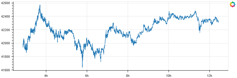
As the data is now inserted into Quasar, we can now query it using the query interface.
We’ll first do a simple plot of all recent trade prices.
q = """
SELECT
$timestamp,
price
FROM
"products/btcusd/trades"
"""
df = qdbpd.query(conn, q)
plot_stock(df, x_axis_type='datetime')
We can turn this data into a classic candlestick OHLC chart in realtime by making using of Quasar’s aggregation functionality. Below is an overview of what Quasar aggregation to use for each of the OHLC features:
Feature |
Function |
|---|---|
Open |
FIRST() |
High |
MAX() |
Low |
MIN() |
Close |
LAST() |
When using aggregation functions, we need to add two conditions to the query:
A “group by” qualifier, that determines what groups to aggregate on. In our case, we will want to specify a time duration, e.g. “5min” if we want OHLC charts with 5 minute buckets;
A timerange qualifier: this tells Quasar the timerange we are interested in, which is required when using aggregations.
The query we will use will look like:
SELECT
$timestamp,
FIRST(price),
MAX(price),
MIN(price),
LAST(price)
FROM ..
IN RANGE <timespan>
GROUP BY <duration>
We can then turn the results of this query into OHLC candlesticks as demonstrated in the code below:
q = """
SELECT
$timestamp,
FIRST(price) AS open,
MAX(price) AS high,
MIN(price) AS low,
LAST(price) AS close
FROM "products/btcusd/trades"
IN RANGE (NOW(), -6h)
GROUP BY 5min
"""
df = qdbpd.query(conn, q).set_index('$timestamp')
plot_ohlc(df)
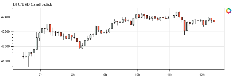
5.2.7. Conclusion#
And that’s all you need to do to get the data in a shape that allows for drawing candlesticks.
In this guide we covered:
How to interact with QuasarDB’s pandas API;
How to create tables, ingest data and query the data;
How to perform aggregations necessary to render OHLC charts.