5.4. Crypto triangular arbitrage using ASOF JOIN#

From Investopedia:

Triangular arbitrage is the result of a discrepancy between three foreign currencies that occurs when the currency’s exchange rates do not exactly match up.

In this guide we are going to see how you can leverage advanced joining capabilities of Quasar to find triangular arbitrage opportunities in cryptocurrencies.

More precisely, in this guide, we will:

Craft a suitable data model for cryptocurrency trade data

Capture and store the data into a Quasar cluster

Query and plot trade data for a single cryptocurrency

Query, align, and plot trade data for multiple single cryptocurrencies

We will be using Python, Pandas, and plotly. You can achieve similar results with any programming language or tool that can query Quasar.

5.4.1. Preparation#

5.4.1.1. Install and launch QuasarDB#

Please install & launch QuasarDB for your environment; the free community edition is sufficient.

For more information and instructions on how to install QuasarDB, please refer to our installation guide.

5.4.1.2. Prepare your Jupyter notebook#

Please follow the steps below to create and set up your Jupyter notebook:

# Install requirements
$ python3 -m pip install jupyter \
                         pandas \
                         numpy \
                         quasardb

# Launch local notebook
$ jupyter notebook ./qdb-howto.ipynb

[I 17:16:02.496 NotebookApp] Serving notebooks from local directory: /home/user/qdb-howto/
[I 17:16:02.496 NotebookApp] Jupyter Notebook 6.4.6 is running at:
[I 17:16:02.496 NotebookApp] http://localhost:8888/?token=...
[I 17:16:02.496 NotebookApp]  or http://127.0.0.1:8888/?token=...
[I 17:16:02.496 NotebookApp] Use Control-C to stop this server and shut down all kernels (twice to skip confirmation).

A new jupyter notebook should automatically open, otherwise please manually navigate and you can navigate your browser to http://localhost:8888/ with the environment prepared.

You are now completed with the preparations.

5.4.2. Triangular arbitrage#

Triangular arbitrage is done by analyzing the discrepancy between three currencies. We will look at USD, BTC, and ETH in our example.

In theory, converting from ETH to USD, should be equivalent to converting from ETH to BTC, and then BTC to USD. However, in carefully analyzing rates, one can find opportunities that result in small, consistent, and low-risk profit.

To find these opportunities, you need to analyze changes in rates and execute trades as soon as the discrepancy is large enough to profit.

This guide will focus on collecting data and ensuring the values are aligned to plot curves of each rate to find arbitrage opportunities. We will not take into account fees.

Warning

This guide is for educational purposes only. In particular, it doesn’t take into account trading fees and relies on trade data. We offer no guarantee regarding its accuracy or completeness.

5.4.3. Getting started#

Coinbase offers a free, public API to pull realtime trade data from. For this demonstration, we will be retrieving realtime trade data for three different pairs:

BTC-USD

ETH-BTC

ETH-USD

Here is how we define a function to load the data for a single symbol into a Pandas Dataframe:

import numpy as np
import pandas as pd
import requests
import io

def pull_coinbase(product, max_pages=25):
    after = None

    xs = list()

    for i in range(max_pages):
        if after is None:
            url = 'https://api.pro.coinbase.com/products/{}/trades'.format(product)
        else:
            url = 'https://api.pro.coinbase.com/products/{}/trades?after={}'.format(product, after)

        r = requests.get(url, timeout=30)
        xs.extend(r.json())

        if not r.headers.get('cb-after'):
            break
        else:
            after = r.headers['cb-after']

    # Convert 'time' column to timezone-naive format
    df = pd.DataFrame(xs)
    df['time'] = pd.to_datetime(df['time']).dt.tz_localize(None)

    dtypes = {'time': np.dtype('datetime64[ns]'),
              'price': np.dtype('float64'),
              'size': np.dtype('float64'),
              'side': np.dtype('U')}

    return df.astype(dtypes).set_index('time').reindex()

We can invoke this function to load BTC-USD symbol data:

btcusd = pull_coinbase('BTC-USD')
btcusd

	trade_id	side	size	price
time
2023-12-06 22:08:59.571599	583806221	buy	0.000628	43916.52
2023-12-06 22:08:59.571599	583806220	buy	0.000372	43916.52
2023-12-06 22:08:59.516604	583806219	buy	0.018400	43916.52
2023-12-06 22:08:57.972088	583806218	sell	0.010839	43916.37
2023-12-06 22:08:57.971081	583806217	buy	0.002289	43914.11
…	…	…	…	…
2023-12-06 20:35:25.073088	583781226	sell	0.009953	44015.73
2023-12-06 20:35:25.068514	583781225	buy	0.043600	44014.39
2023-12-06 20:35:25.058233	583781224	buy	0.068242	44015.72
2023-12-06 20:35:24.958960	583781223	buy	0.043600	44017.20
2023-12-06 20:35:24.923809	583781222	buy	0.069991	44017.54

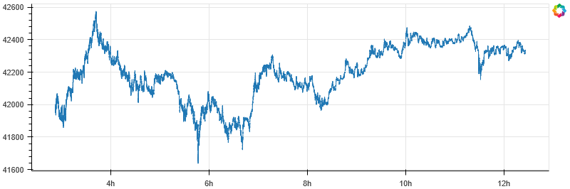
This data looks like this:

import plotly.express as px
fig = px.line(x=btcusd.index, y=btcusd.price)
fig.update_layout(template='plotly_dark',
                  title='BTC-USD')

fig.show()

Before we can get started with ingesting this data into Quasar, we must import the required libraries and establish a connection with the database.

5.4.4. Writing to Quasar#

import quasardb
import quasardb.pandas as qdbpd

conn = quasardb.Cluster('qdb://127.0.0.1:2836')
conn

<quasardb.quasardb.Cluster at 0x7f33cb3f35b0>

The QuasarDB pandas API, imported as qdbpd, has a write_dataframe function we can leverage to store a Pandas dataframe directly into QuasarDB. The following code shows you how to use it to write the data the dataframe into a table called btcusd:

table = conn.table('btcusd')
qdbpd.write_dataframe(btcusd,
                      conn,
                      table,
                      # Automatically create the table if not found
                      create=True)

In addition to writing (and reading) dataframes from entire tables, the QuasarDB pandas API exposes the query function which can be used to use our query language. For example, we can select all data from the btcusd table using the following query:

SELECT * FROM btcusd

In Pandas, we can do this as follows:

df = qdbpd.query(conn, "SELECT * FROM btcusd")
df

	$timestamp	$table	trade_id	side	size	price
0	2023-12-06 20:35:24.923809	btcusd	583781222	buy	0.069991	44017.54
1	2023-12-06 20:35:24.958960	btcusd	583781223	buy	0.043600	44017.20
2	2023-12-06 20:35:25.058233	btcusd	583781224	buy	0.068242	44015.72
3	2023-12-06 20:35:25.068514	btcusd	583781225	buy	0.043600	44014.39
4	2023-12-06 20:35:25.073088	btcusd	583781226	sell	0.009953	44015.73
…	…	…	…	…	…	…
24995	2023-12-06 22:08:57.971081	btcusd	583806217	buy	0.002289	43914.11
24996	2023-12-06 22:08:57.972088	btcusd	583806218	sell	0.010839	43916.37
24997	2023-12-06 22:08:59.516604	btcusd	583806219	buy	0.018400	43916.52
24998	2023-12-06 22:08:59.571599	btcusd	583806220	buy	0.000372	43916.52
24999	2023-12-06 22:08:59.571599	btcusd	583806221	buy	0.000628	43916.52

As you can see above, the trade data is indeed available in this table.

We now have loaded the data into Quasar. We can repeat this process for the two other products we want to track, ETH-USD and ETH-BTC:

xs = [('ethusd', 'ETH-USD'),
      ('ethbtc', 'ETH-BTC')]

for (tablename, symbol) in xs:
    qdbpd.write_dataframe(pull_coinbase(symbol),
                          conn,
                          conn.table(tablename),
                          create=True)

So now we have three tables: btcusd, ethusd and ethbtc.

We can use an asof join between these tables as follows:

SELECT
  "$timestamp",
  btcusd.price * ethbtc.price AS btcethusd,
  ethusd.price AS ethusd
FROM btcusd
LEFT ASOF JOIN ethusd, ethbtc

This will instruct QuasarDB to join the data as follows:

For each row of btcusd, get the $timestamp.
Look for the last known price inside ethusd as of $timestamp
Look for the last known price inside ethbtc as of $timestamp
Calculate the price of acquiring ETH by first buying BTC for USD and then acquiring ETH for BTC;
Merge the results into a single row.

This will then return a dataframe that looks like this:

import plotly.graph_objects as go

q = """
SELECT
  $timestamp,
  btcusd.price * ethbtc.price AS btcethusd,
  ethusd.price AS ethusd
FROM ethusd
LEFT ASOF JOIN btcusd, ethbtc
WHERE
  price IS NOT NULL
"""
df = qdbpd.query(conn, q).set_index('$timestamp').reindex()

fig = go.Figure()
fig.add_trace(go.Scatter(x=df.index, y=df['btcethusd'], name='ETH-BTC-USD'))
fig.add_trace(go.Scatter(x=df.index, y=df['ethusd'], name='ETH-USD'))
fig.update_layout(template='plotly_dark',
                  title='ETH-USD vs ETH-BTC-USD')
fig.show()

5.4.5. Conclusion#

Aligning timeseries is crucial for many financial analyses, and triangular arbitrage is no exception.

Thanks to the built-in support for ASOF JOINS, Quasar enables you to quickly and efficiently join multiple timeseries.

The approach we used in this guide will work for any timeseries dataset; Quasar will optimize the query on the fly.

5.4.5.1. Further readings#

Creating OHLC charts with Quasar

../api/tutorial

Select