5.6. How to handle multiple versions of the same data

Let’s say you’re working on forecast data and that this forecast data is updated multiple times a day.

While it could be tempting to “update” the value in your database to the latest forecast (and keep only that), you may be interested in maintaining all versions.

For example, you may want to evaluate the accuracy of the different forecasts. In trading, another reason could be to do backtesting with the forecast value “as it was”.

How to maintain multiple versions of a value?

In this guide, we will:

• See how you can model data to support multiple versions of a value for a given timestamp

• How to query a specific version of the data present in the database

• How to render a specific version of the data in a curve

We will be using Python, Pandas, and plotly. You can achieve similar results with any programming language or tool that can query Quasar.

5.6.1. Preparation

5.6.1.1. Install and launch QuasarDB

Please install & launch QuasarDB for your environment; the free community edition is sufficient.

For more information and instructions on how to install QuasarDB, please refer to our installation guide.

5.6.1.2. Prepare your Jupyter notebook

Please follow the steps below to create and set up your Jupyter notebook:

# Install requirements
$ python3 -m pip install jupyter \
                         pandas \
                         numpy \
                         quasardb

# Launch local notebook
$ jupyter notebook ./qdb-howto.ipynb

[I 17:16:02.496 NotebookApp] Serving notebooks from local directory: /home/user/qdb-howto/
[I 17:16:02.496 NotebookApp] Jupyter Notebook 6.4.6 is running at:
[I 17:16:02.496 NotebookApp] http://localhost:8888/?token=...
[I 17:16:02.496 NotebookApp]  or http://127.0.0.1:8888/?token=...
[I 17:16:02.496 NotebookApp] Use Control-C to stop this server and shut down all kernels (twice to skip confirmation).

A new jupyter notebook should automatically open, otherwise please manually navigate and you can navigate your browser to http://localhost:8888/ with the environment prepared.

You are now completed with the preparations.

5.6.2. Modeling multiple versions

Let’s say we’re tasked with storing temperature forecasts with the requirements:

• Forecasts are made on a daily basis;

• Each forecast describes the day ahead and the 7 days following;

• Each forecast has data points in intervals of 1 hour;

• We want to keep track of the entire history of all forecasts, i.e. old forecasts will never be deleted;

• When querying data, we typically want to use only the most recent forecast.

We can generate data for a single forecast as follows:

import math
import numpy as np
import pandas as pd

basetime = np.datetime64('2021-09-01')
basetemp = 18
d = 0.05
def temp_for(i):
    # semi-natural temperature forecast
    t = basetemp / float(i + 1)
    return basetemp * (math.exp(-d/t))

def gen_forecast(start):
    offset = (start - basetime) / np.timedelta64(1, 'h')
    return [{'When': start + np.timedelta64(i, 'h'),
             'Forecast made at': start,
             'Temperature': temp_for(i) + offset} for i in range(0, (24 * 60))]

df = pd.DataFrame(data=gen_forecast(basetime))
df

	When	Forecast made at	Temperature
0	2021-09-01 00:00:00	2021-09-01	17.950069
1	2021-09-01 01:00:00	2021-09-01	17.900277
2	2021-09-01 02:00:00	2021-09-01	17.850623
3	2021-09-01 03:00:00	2021-09-01	17.801107
4	2021-09-01 04:00:00	2021-09-01	17.751728
…	…	…	…
1435	2021-10-30 19:00:00	2021-09-01	0.333365
1436	2021-10-30 20:00:00	2021-09-01	0.332440
1437	2021-10-30 21:00:00	2021-09-01	0.331518
1438	2021-10-30 22:00:00	2021-09-01	0.330599
1439	2021-10-30 23:00:00	2021-09-01	0.329681

In order to model this data, we can observe the following:

• As the column When describes the time the data point describes, and is most likely to be queried for, we use this as our primary $timestamp index;

• We can use Forecast made at to find the most recent forecast for a query: it effectively describes the version of the data.

In other words, this data is bitemporal: one timestamp describing the time/temperature being forecasted, and another timestamp of when the forecast itself was made.

In Quasar, we can store the data as-is, in a table with three columns:

• The primary $timestamp index;

• A version timestamp column;

• A temperature double column.

5.6.3. Writing to Quasar

We can take this forecast data and write it to Quasar.

Let’s first establish a connection with Quasar and create the table:

import quasardb
import quasardb.pandas as qdbpd

conn = quasardb.Cluster('qdb://127.0.0.1:2836')
table = conn.table('forecasts')

try:
   table.remove()
except:
   # Table did not yet exist
   pass

cols = [quasardb.ColumnInfo(quasardb.ColumnType.Timestamp, "version"),
        quasardb.ColumnInfo(quasardb.ColumnType.Double, "temperature")]

table.create(cols)

Let’s generate 3 different forecasts, and insert them into Quasar:

def insert_forecast(forecast):
  # Convert to DataFrame
  df = pd.DataFrame(data=forecast)
  df = df.rename(columns={'When': '$timestamp', 'Forecast made at': 'version', 'Temperature': 'temperature'})
  df = df.round({'temperature': 3})
  df = df.set_index('$timestamp').reindex()

  # Invoke QuasarDB Pandas API to store this forecast
  qdbpd.write_dataframe(df, conn, table)

# Generate 10 forecasts, one for each hour starting at 2021-09-01
timestamps = (basetime + np.timedelta64(i, 'h') for i in range(10))
forecasts = [gen_forecast(np.datetime64(timestamp)) for timestamp in timestamps]

# Use first 3 forecasts
for forecast in forecasts[:3]:
   insert_forecast(forecast)

5.6.4. How to query the data

We can retrieve the first 10 rows of the data by using a simple Quasar query for the QuasarDB pandas API:

q = "SELECT $timestamp, version, temperature FROM forecasts ORDER BY $timestamp LIMIT 10"
df = qdbpd.query(conn, q)
df

	$timestamp	version	temperature
0	2021-09-01 00:00:00	2021-09-01 00:00:00	17.950
1	2021-09-01 01:00:00	2021-09-01 00:00:00	17.900
2	2021-09-01 01:00:00	2021-09-01 01:00:00	18.950
3	2021-09-01 02:00:00	2021-09-01 00:00:00	17.851
4	2021-09-01 02:00:00	2021-09-01 01:00:00	18.900
5	2021-09-01 02:00:00	2021-09-01 02:00:00	19.950
6	2021-09-01 03:00:00	2021-09-01 00:00:00	17.801
7	2021-09-01 03:00:00	2021-09-01 01:00:00	18.851
8	2021-09-01 03:00:00	2021-09-01 02:00:00	19.900
9	2021-09-01 04:00:00	2021-09-01 00:00:00	17.752

As you can see above, we indeed have all the data in the database, and it should be apparant that we indeed have 3 versions of the data.

In order to focus on a single version, your intuition might be to make a query with a WHERE clause specifying a specific version number or a specific forecast time. For example, the following could work:

version = "2021-09-01T05:00:00"
q = """
SELECT
  $timestamp,
  version,
  temperature

FROM forecasts
WHERE version = DATETIME({})
""".format(version)
df = qdbpd.query(conn, q)
df

	0

This is all well and good, but what if not every row has the same version of the forecast? In the data above we’re missing the first few rows, because of this reason.

Often, what we’re interested in is “the last version of the forecast available, whatever that is”, but we don’t know the exact version timestamp.

Fortunately, Quasar has a built-in query for this with the RESTRICT TO keyword. The RESTRICT TO keyword will restrict the query to a specific “version” based on the value of a given column.

In our example, if we want to have the “last version” of the forecast available, whatever that is, the query becomes:

q = """
SELECT
  $timestamp,
  version,
  temperature

FROM forecasts
RESTRICT TO MAX(version)
"""
df = qdbpd.query(conn, q)
df

	$timestamp	version	temperature
0	2021-09-01 00:00:00	2021-09-01 00:00:00	17.950
1	2021-09-01 01:00:00	2021-09-01 01:00:00	18.950
2	2021-09-01 02:00:00	2021-09-01 02:00:00	19.950
3	2021-09-01 03:00:00	2021-09-01 02:00:00	19.900
4	2021-09-01 04:00:00	2021-09-01 02:00:00	19.851
…	…	…	…
1437	2021-10-30 21:00:00	2021-09-01 02:00:00	2.333
1438	2021-10-30 22:00:00	2021-09-01 02:00:00	2.332
1439	2021-10-30 23:00:00	2021-09-01 02:00:00	2.332
1440	2021-10-31 00:00:00	2021-09-01 02:00:00	2.331
1441	2021-10-31 01:00:00	2021-09-01 02:00:00	2.330

As you can see, here it automatically does the right thing: for the first few rows, it uses the last available forecast at that time.

5.6.5. Point in Time

There is an additional advantage to using timestamped versions: it allows us to reconstruct the data as of a certain time. This is very useful functionality to back-test algorithms, resolve quality issues, and/or help with auditing.

To achieve this, we take the following steps:

• Before filtering for the most recent version, apply a WHERE clause that removes any rows with a version after a certain date;

• Use the same RESTRICT TO syntax as described above to keep only the most recent version.

If, for example, we want to figure out what the state of the database is at 2021-09-01T01:15, we can do so as follows:

q = """
SELECT
  $timestamp,
  version,
  temperature

FROM forecasts
WHERE version <= DATETIME(2021-09-01T01:15)
RESTRICT TO MAX(version)
"""
df = qdbpd.query(conn, q)
df

	$timestamp	version	temperature
0	2021-09-01 00:00:00	2021-09-01 00:00:00	17.95
1	2021-09-01 01:00:00	2021-09-01 01:00:00	18.95

As you can see, it now returns the data as it was at that exact point in time.

5.6.6. Plotting multiple versions

Of course, we can use this data to plot multiple versions in the same chart. This can be very useful to visualize the behavior of a forecasting algorithm over time.

Let’s start out with plotting multiple versions as multiple lines in a chart. We’ll be using plotly for these visualizations.

import plotly.graph_objects as go

q = """
SELECT
  $timestamp,
  version,
  temperature

FROM forecasts

IN RANGE (2021-09-03T00:00:00, +1month)
"""
df = qdbpd.query(conn, q).set_index('$timestamp').reindex()
groups = df.groupby('version', axis=0)

fig = go.Figure()
for (version, df_) in groups:
  fig.add_trace(go.Scatter(x=df_.index, y=df_['temperature'], name='version={}'.format(str(version))))

fig.update_layout(template='plotly_dark')
fig.show()

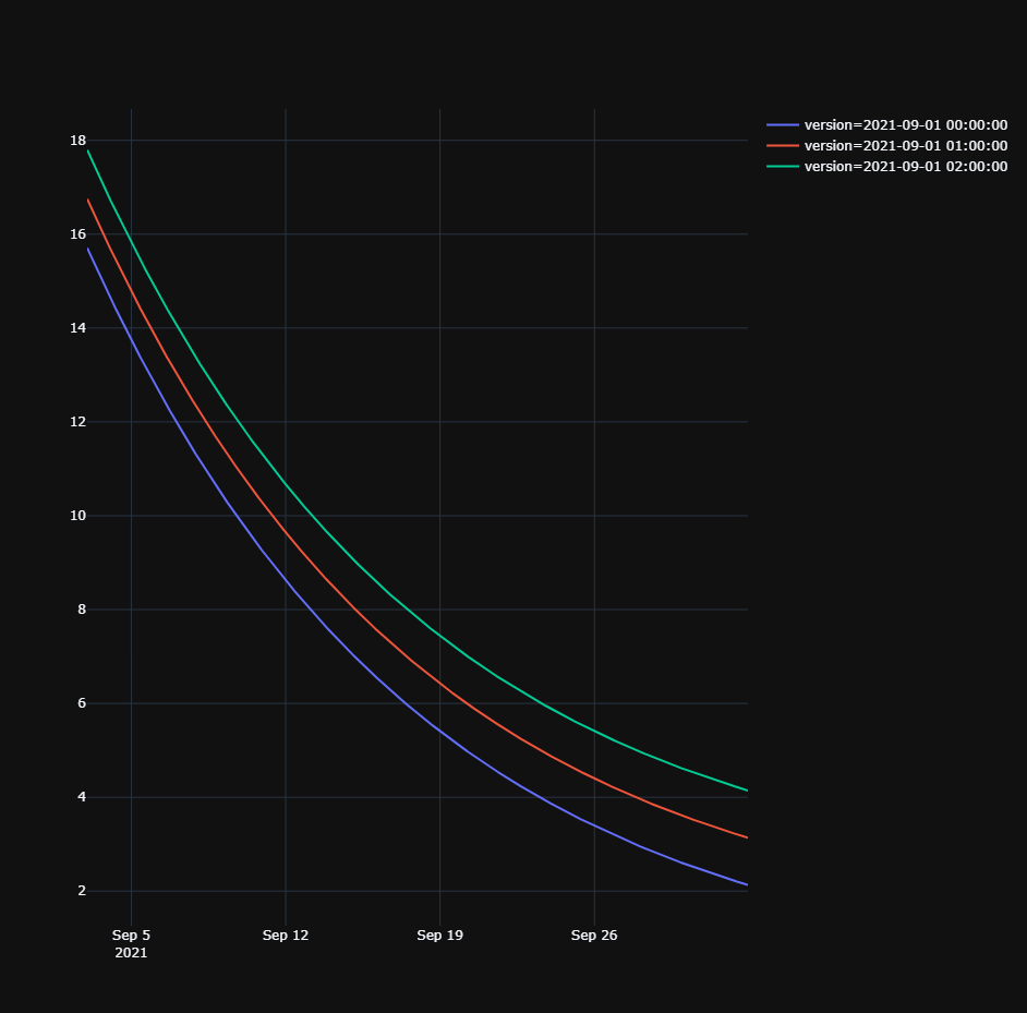
If we have many different forecasts, it also allows you to zoom in into specific timeslots and observe the forecasts over time.

Let’s first insert the remaining forecasts:

# Insert the rest of the forecasts
for forecast in forecasts[3:]:
   insert_forecast(forecast)

And now we can zoom in into a single timeslot and plot the forecasts over time.

import plotly.graph_objects as go

q = """
SELECT
  $timestamp,
  version,
  temperature

FROM forecasts

IN RANGE (2021-09-14T00:00:00, +1h)
"""
df = qdbpd.query(conn, q).set_index('$timestamp').reindex()

fig = go.Figure()
fig.add_bar(x=df['version'], y=df['temperature'])
fig.update_layout(template='plotly_dark')
fig.show()

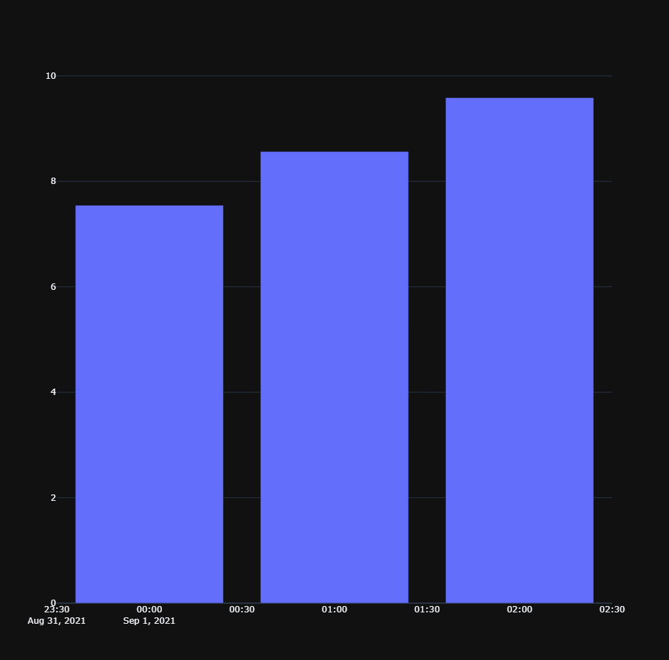
In this chart, the x-axis is the version of the forecast, and the y-axis is the forecasted temperature.

As all forecasted values are about the exact same time slot, a chart like this allows us to compare the accuracy of the forecasting over time.

5.6.7. Conclusion

In this tutorial you learned:

• how to use a timestamp to store versioned data in Quasar;

• how to query data based for a specific version;

• how to query data based for the most recent version available;

• how to use the version timestamp to reconstruct the state of the database as of a certain point in time.

5.6.7.1. Further readings

• ../api/tutorial

• Reaching your performance goals