5.1. Industrial waveform processing with Quasar#

In industrial manufacturing, electrical and mechanical waveforms are captured for real-time monitoring and analytical purposes. This allows the operators to predict and prevent issues before they occur.

In this guide we will walk through a typical waveform use case, which will cover:

Modeling waveform data with Quasar;

Transforming raw waveform payload;

Using the Quasar Pandas API for ingestion and querying.

Completing this guide will take 30-60 minutes.

5.1.1. Preparation#

If you wish to run this guide locally, there are two ways to prepare your local development environment:

5.1.1.1. Docker#

We have prepared a pre-loaded Docker image which contains everything needed to run practice guide. To get started, please launch the bureau14/howto-iot-waveform Docker container as follows:

$ docker run -ti --net host bureau14/iot-waveform:3.13.0
Launching QuasarDB in background..
Launching Jupyter lab...
[I 13:20:59.346 NotebookApp] Writing notebook server cookie secret to /home/qdb/.local/share/jupyter/runtime/notebook_cookie_secret
[I 13:20:59.501 NotebookApp] Serving notebooks from local directory: /work/notebook
[I 13:20:59.501 NotebookApp] Jupyter Notebook 6.4.6 is running at:
[I 13:20:59.501 NotebookApp] http://localhost:8888/?token=...
[I 13:20:59.501 NotebookApp]  or http://127.0.0.1:8888/?token=...

You can now navigate with your browser to the URL provided by the Jupyter notebook and continue with this exercise.

5.1.1.2. Standalone installation#

5.1.1.2.1. Install and launch QuasarDB#

Please install & launch QuasarDB for your environment; the free community edition is sufficient.

For more information and instructions on how to install QuasarDB, please follow our installation guide.

5.1.1.2.2. Download this Jupyter notebook#

You can download this notebook prepackaged from this location:

iot-waveform-env.tar.gz

Please download this, and extract it in a folder on your local machine.

5.1.1.2.3. Prepare Python environment#

# Create virtualenv
$ python3 -m venv .env/

$ source .env/bin/activate

# Install requirements
(.env)
$ python3 -m pip install -r requirements.txt

# Launch local notebook
(.env)
$ jupyter notebook ./iot-waveform.ipynb

[I 17:16:02.496 NotebookApp] Serving notebooks from local directory: /home/user/qdb-guides/
[I 17:16:02.496 NotebookApp] Jupyter Notebook 6.4.6 is running at:
[I 17:16:02.496 NotebookApp] http://localhost:8888/?token=...
[I 17:16:02.496 NotebookApp]  or http://127.0.0.1:8888/?token=...
[I 17:16:02.496 NotebookApp] Use Control-C to stop this server and shut down all kernels (twice to skip confirmation).

A new jupyter notebook should automatically open, otherwise please manually navigate and you can navigate your browser to http://localhost:8888/ with the environment prepared.

You are now completed with the preparations.

5.1.2. Electrical waveform#

In this tutorial, we will be working with 3-phase electrical waveform data. This is a common type of data collected for industrial manufacturing.

According to the Wikipedia page about Three-phase electric power

Three-phase power works by the voltage and currents being 120 degrees out of phase on the three wires. As an AC system it allows the voltages to be easily stepped up using transformers to high voltage for transmission, and back down for distribution, giving high efficiency.

A three-wire three-phase circuit is usually more economical than an equivalent two-wire single-phase circuit at the same line to ground voltage because it uses less conductor material to transmit a given amount of electrical power. Three-phase power is mainly used directly to power large motors and other heavy loads. Small loads often use only a two-wire single-phase circuit, which may be derived from a three-phase system.

As such, industrial manufacturers use 3-phrase electricity for their heavy equipment.

In order to prevent problems and potential breakdowns of this equipment, the electricity is monitored for several purposes:

Detect and mitigate surges / sags;

Build predictive maintenance models to detect early signals of machine failure;

Analyze specific historical moments of interest to better understand the behavior of their equipment.

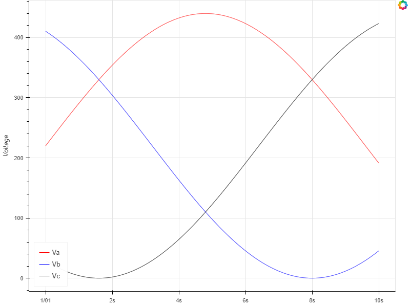
For this, measurement devices are added to the electrical circuits that capture the measurements. Such measurements are represented using waveforms, and looks like this:

import pandas as pd
from utils import sine
from utils import plot_waveform

df = pd.DataFrame({'vA': sine(0, 200, 5, 500),
                'vB': sine(120, 200, 5, 500),
                'vC': sine(240, 200, 5, 500)})
_ = plot_waveform(df)

In this example above, you can see all three phases identified by colors (red, blue and black).

The data captured has the following configuration:

Both voltage and current are measured;

Each phase is measured individually. This means that for each measurement, we get 6 data points, voltage and current for each of the three phases.

The frequency is 50Hz or 60Hz, depending on the country;

Sampling rate is typically between 40,000 and 80,000 samples per second.

Continuously monitoring all electricity would be a rather costly operation: a single machine with two sensors generates over 3 billion data points in 12 hours of operation, and the majority of that data would not be that interesting.

Instead, data is captured during a short period, typically 30s - 60s, at moments of interest: typically at machine start / machine stop. The data for a single measurement period is captured and aggregated as a single unit, which we call “payload”.

In this tutorial, we will be focus heavily on the capturing, processing and analysis of these payloads.

5.1.3. Imports and setups#

Now that we have explained what electrical waveform data is, we can start working on the actual solution.

First let’s go through some boilerplate to import libraries and establish a connection with the QuasarDB cluster.

import datetime
import json
import random
import pprint
import copy
from tqdm import tqdm

import numpy as np
import pandas as pd
import quasardb
import quasardb.pandas as qdbpd

# Utilities for plotting waveforms
from utils import plot_waveform
pp = pprint.PrettyPrinter(indent=2, sort_dicts=False)


def get_conn():
    return quasardb.Cluster("qdb://127.0.0.1:2836")

# This connection will be used for the remainder of the notebook
conn = get_conn()

5.1.4. Load sample data#

Loads all sample waveform data that is used for this guide. It will be available in the payloads dict.

from io import BytesIO
from gzip import GzipFile
from urllib.request import urlopen, Request
import tarfile

resp = urlopen(Request("https://doc.quasardb.net/howto/iot-waveform/iot-waveform-data.tar.gz", headers={'User-Agent': 'Mozilla/5.0'}))
f = GzipFile(fileobj=BytesIO(resp.read()))
tf = tarfile.TarFile(fileobj=f)
files = tf.getmembers()

n = 0
payloads = []
for file in files:
    fn = file.name

    with tf.extractfile(fn) as fp:
        payload = json.loads(fp.read())
        for k in payload['axis'].keys():
            n += len(payload['axis'][k])

        payloads.append(payload)

print("Loaded {} waveform payloads with a total of {:,} points ({:,} per payload)".format(len(payloads), n, int(n / len(payloads))))

Loaded 15 waveform payloads with a total of 17,280,000 points (1,152,000 per payload)

5.1.5. Waveform capture#

A typical waveform ingestion process is as follows:

A device measures a for a brief period, and captures values at a predefined interval (e.g. 20,000 Hz).
This data is compressed into a single payload with an associated timestamp and sensor id.
It is then uploaded to be processed and ingested into the main database.

An example of an electrical waveform payload may look like this as it arrives:

payload = copy.deepcopy(payloads[0])
# Truncate the payload slightly for readability
for k in payload['axis'].keys():
    payload['axis'][k] = payload['axis'][k][0:5]
payload['count'] = 5

pp.pprint(payload)


p = payloads[0]
per_cycle = int(p['sample_rate'] / p['freq'])
n_cycles = 5

print()
print("Voltage waveform visualization (first {} cycles, with a resolution of {:,} points per cycle)".format(n_cycles, per_cycle))
print()

df = pd.DataFrame(p['axis'], columns=['volt-a', 'volt-b', 'volt-c'])
df = df[0:(per_cycle * n_cycles)]
_ = plot_waveform(df, xaxis_label='Samples (n)')

{ 'timestamp': '2021-09-12T12:03:03',
'payload_id': 0,
'sensor_id': 'emea-fac1-elec-1832',
'sample_count': 192000,
'sample_rate': 48000,
'freq': 5,
'axis': { 'volt-a': [ 220.0,
                        220.07199483035976,
                        220.14398965300944,
                        220.21598446023896,
                        220.28797924433826],
            'volt-b': [ 410.52558883257655,
                        410.48958121550766,
                        410.45355319851706,
                        410.41750478546294,
                        410.3814359802059],
            'volt-c': [ 29.47441116742357,
                        29.438423954132645,
                        29.402457148473616,
                        29.36651075429822,
                        29.33058477545589],
            'cur-a': [ 220.0,
                    220.07199483035976,
                    220.14398965300944,
                    220.21598446023896,
...
'count': 5}

Voltage waveform visualization (first 5 cycles, with a resolution of 9,600 points per cycle)

We can observe a few things from this data:

We have 6 axis per payload (voltage A/B/C, current A/B/C)
Data is packed in a columnar fashion;
Each payload is identified with a unique payload_id;
We don’t have timestamps for each of the points in the axis.
We have the sample rate (how many samples / sec), sample count (total number of samples per axis) and frequency (50 Hz).

Let’s see how we model this data in Quasar.

5.1.6. Data modelling#

In Quasar, we represent waveform data as follows:

We create a table per sensor;

We pivot all the payload axis, such that the different voltages / currents are on the same row;

We assign an absolute timestamp to each of the rows.

To do this, we create a table as follows:

def create_table(conn, sensor_id):
    cols = [quasardb.ColumnInfo(quasardb.ColumnType.String, "sensor_id"),
            quasardb.ColumnInfo(quasardb.ColumnType.Int64, "payload_id"),
            quasardb.ColumnInfo(quasardb.ColumnType.Int64, "sample_count"),
            quasardb.ColumnInfo(quasardb.ColumnType.Int64, "sample_rate"),
            quasardb.ColumnInfo(quasardb.ColumnType.Int64, "freq"),
            quasardb.ColumnInfo(quasardb.ColumnType.Double, "Va"),
            quasardb.ColumnInfo(quasardb.ColumnType.Double, "Ia"),
            quasardb.ColumnInfo(quasardb.ColumnType.Double, "Vb"),
            quasardb.ColumnInfo(quasardb.ColumnType.Double, "Ib"),
            quasardb.ColumnInfo(quasardb.ColumnType.Double, "Vc"),
            quasardb.ColumnInfo(quasardb.ColumnType.Double, "Ic")]

    # Assumes `conn` is an existing connection to the Quasar cluster
    try:
        conn.table(sensor_id).create(cols, datetime.timedelta(seconds=1))
    except quasardb.AliasAlreadyExistsError:
        pass

create_table(conn, payload['sensor_id'])
# Let's verify the table exists and query its columns
conn.table(payload['sensor_id']).list_columns()

[<quasardb.ColumnInfo name='sensor_id' type='string'>,
<quasardb.ColumnInfo name='payload_id' type='int64'>,
<quasardb.ColumnInfo name='sample_count' type='int64'>,
<quasardb.ColumnInfo name='sample_rate' type='int64'>,
<quasardb.ColumnInfo name='freq' type='int64'>,
<quasardb.ColumnInfo name='Va' type='double'>,
<quasardb.ColumnInfo name='Ia' type='double'>,
<quasardb.ColumnInfo name='Vb' type='double'>,
<quasardb.ColumnInfo name='Ib' type='double'>,
<quasardb.ColumnInfo name='Vc' type='double'>,
<quasardb.ColumnInfo name='Ic' type='double'>]

We have now created our table, and verified it succeeded by retrieving its schema from the database. Our next task is to transform the raw waveform payload into this model.

5.1.7. Data transformation#

To transform the data, we need to perform the following tasks:

Based on sample_rate, determine the time delta between each of the points; e.g. if sample_rate is 100, it means that the time delta between each of the points is 1s / 100 = 10ms.
Pivot all the axis, such that the points for Va, Ia, Vb, etc are on the same row;
Based on the input timestamp and timedelta, calculate the absolute timestamp for each of the rows.

The code below achieves this.

def transform_payload(payload):
    start_time = np.datetime64(payload['timestamp'], 'ns')

    sensor_id = payload['sensor_id']
    payload_id = payload['payload_id']
    wav_n = payload['sample_count']
    wav_rate = payload['sample_rate']

    # Validation: ensure that each of the axis has exactly `count` points.
    for axis in payload['axis'].keys():
        assert len(payload['axis'][axis]) == wav_n

    # Create the base dict for all our axis
    m = {'Va': payload['axis']['volt-a'],
        'Ia': payload['axis']['cur-a'],
        'Vb': payload['axis']['volt-b'],
        'Ib': payload['axis']['cur-b'],
        'Vc': payload['axis']['volt-c'],
        'Ic': payload['axis']['cur-c']}

    # Using the timestamp and frequency, we can calculate the timestamps for each of
    # the rows.
    timedelta = np.timedelta64(1000000000, 'ns') / wav_rate
    timestamps = [(start_time + (timedelta * i)) for i in range(wav_n)]

    # Create arrays for sensor/count/freq, which always contain the same value
    m['sensor_id'] = np.repeat(sensor_id, (wav_n))
    m['payload_id'] = np.repeat(payload_id, (wav_n))

    for col in payload.keys():
        if col != 'axis':
            m[col] = np.repeat(payload[col], (wav_n))

    # And represent the transformation result as a Python DataFrame
    df = pd.DataFrame(index=timestamps,
                    data=m,
                    columns=['sensor_id', 'payload_id', 'sample_rate', 'sample_count', 'freq', 'Va', 'Ia', 'Vb', 'Ib', 'Vc', 'Ic'])
    return (sensor_id, payload_id, df)

(sensor_id, payload_id, df) = transform_payload(payloads[0])

df

	sensor_id	payload_id	sample_rate	sample_count	freq	Va	Ia	Vb	Ib	Vc	Ic
2021-09-12 12:03:03.000000000	emea-fac1-elec-1832	0	48000	192000	5	220.000000	220.000000	410.525589	410.525589	29.474411	29.474411
2021-09-12 12:03:03.000020833	emea-fac1-elec-1832	0	48000	192000	5	220.071995	220.071995	410.489581	410.489581	29.438424	29.438424
2021-09-12 12:03:03.000041666	emea-fac1-elec-1832	0	48000	192000	5	220.143990	220.143990	410.453553	410.453553	29.402457	29.402457
2021-09-12 12:03:03.000062499	emea-fac1-elec-1832	0	48000	192000	5	220.215984	220.215984	410.417505	410.417505	29.366511	29.366511
2021-09-12 12:03:03.000083332	emea-fac1-elec-1832	0	48000	192000	5	220.287979	220.287979	410.381436	410.381436	29.330585	29.330585
…	…	…	…	…	…	…	…	…	…	…	…
2021-09-12 12:03:06.999831835	emea-fac1-elec-1832	0	48000	192000	5	219.640026	219.640026	410.705321	410.705321	29.654653	29.654653
2021-09-12 12:03:06.999852668	emea-fac1-elec-1832	0	48000	192000	5	219.712021	219.712021	410.669415	410.669415	29.618564	29.618564
2021-09-12 12:03:06.999873501	emea-fac1-elec-1832	0	48000	192000	5	219.784016	219.784016	410.633489	410.633489	29.582495	29.582495
2021-09-12 12:03:06.999894334	emea-fac1-elec-1832	0	48000	192000	5	219.856010	219.856010	410.597543	410.597543	29.546447	29.546447
2021-09-12 12:03:06.999915167	emea-fac1-elec-1832	0	48000	192000	5	219.928005	219.928005	410.561576	410.561576	29.510419	29.510419

As you can see, we have achieved our goals:

All waveform points have an associated absolute timestamp;
The timestamps are derived from the sample rate (48,000 Hz ~= 0.00002s per sample);
All points are aligned on rows based on the timestamp.

Let’s transform all the remaining payloads, so that all data is in the correct shape to ingest into Quasar.

payloads_transformed = [transform_payload(payload) for payload in tqdm(payloads)]

100%|██████████████████████████████| 15/15 [00:14<00:00,  1.01it/s]

5.1.8. Ingestion#

As we have all the building blocks together now, let’s define the function that ingests our payloads. As we use Pandas before, we can use the Quasar Pandas API directly to insert the data into Quasar.

def ingest_payload(conn, sensor_id, df):
    table = conn.table(sensor_id)

    qdbpd.write_pinned_dataframe(df, conn, table, create=False, fast=True, infer_types=False)

create_table(conn, sensor_id)
ingest_payload(conn, sensor_id, df)

5.1.8.1. Ingest everything#

Let’s apply this ingestion function to all our payloads and ingest everything into Quasar

# We can apply this function for all our waveforms!
sensor_ids = set()

for (sensor_id, payload_id, df) in tqdm(payloads_transformed[1:]):
    if not sensor_id in sensor_ids:
        create_table(conn, sensor_id)
        sensor_ids.add((sensor_id, payload_id))

    ingest_payload(conn, sensor_id, df)

100%|██████████████████████████████| 15/15 [00:14<00:00,  1.01it/s]

And with this, we have successfully completed an ETL process to ingest waveform data into Quasar.

So far, we have covered:

The shape of raw waveform data;

How to model this data in Quasar;

Transforming raw waveform data into the correct shape for Quasar;

Ingestion into Quasar using the Pandas API.

5.1.9. Retrieving data#

Now that we have the data into Quasar, we will want to query it. We will be using the Pandas API again to query the data directly into dataframes.

5.1.9.1. Pandas query APIs#

There are two ways in which we can retrieve data from Quasar using the Pandas API:

Use qdbpd.read_dataframe to read all data of a table into a DataFrame. If you are looking to retrieve all data of a table (or in a range), this function provides you with the best performance for the task.

Use qdbpd.query to execute a server-side query, and return the results as a DataFrame.

Let’s first use the read_dataframe function to read all data from the waveform table.

# Use the `read_dataframe` function to read all waveform data into a single
# dataframe, to verify all data is ingested.

sensor_id = payloads[1]['sensor_id']

table = conn.table(sensor_id)
df = qdbpd.read_dataframe(table)
df

	sensor_id	payload_id	sample_count	sample_rate	freq	Va	Ia	Vb	Ib	Vc	Ic
2021-09-12 12:06:03.000000000	emea-fac1-elec-1839	1	192000	48000	5	220.000000	220.000000	410.525589	410.525589	29.474411	29.474411
2021-09-12 12:06:03.000020833	emea-fac1-elec-1839	1	192000	48000	5	220.071995	220.071995	410.489581	410.489581	29.438424	29.438424
2021-09-12 12:06:03.000041666	emea-fac1-elec-1839	1	192000	48000	5	220.143990	220.143990	410.453553	410.453553	29.402457	29.402457
2021-09-12 12:06:03.000062499	emea-fac1-elec-1839	1	192000	48000	5	220.215984	220.215984	410.417505	410.417505	29.366511	29.366511
2021-09-12 12:06:03.000083332	emea-fac1-elec-1839	1	192000	48000	5	220.287979	220.287979	410.381436	410.381436	29.330585	29.330585
…	…	…	…	…	…	…	…	…	…	…	…
2021-09-12 12:13:42.999831835	emea-fac1-elec-1839	6	192000	48000	5	219.640026	219.640026	410.705321	410.705321	29.654653	29.654653
2021-09-12 12:13:42.999852668	emea-fac1-elec-1839	6	192000	48000	5	219.712021	219.712021	410.669415	410.669415	29.618564	29.618564
2021-09-12 12:13:42.999873501	emea-fac1-elec-1839	6	192000	48000	5	219.784016	219.784016	410.633489	410.633489	29.582495	29.582495
2021-09-12 12:13:42.999894334	emea-fac1-elec-1839	6	192000	48000	5	219.856010	219.856010	410.597543	410.597543	29.546447	29.546447
2021-09-12 12:13:42.999915167	emea-fac1-elec-1839	6	192000	48000	5	219.928005	219.928005	410.561576	410.561576	29.510419	29.510419

5.1.9.2. Specifying columns#

If we only care about a few column, we can speed up the performance even more by selecting less columns. As Quasar is a column-oriented database, selecting a subset of columns is very efficient and encouraged.

df = qdbpd.read_dataframe(table, columns=['payload_id', 'Va', 'Vb', 'Vc'])
df

	payload_id	Va	Vb	Vc
2021-09-12 12:06:03.000000000	1	220.000000	410.525589	29.474411
2021-09-12 12:06:03.000020833	1	220.071995	410.489581	29.438424
2021-09-12 12:06:03.000041666	1	220.143990	410.453553	29.402457
2021-09-12 12:06:03.000062499	1	220.215984	410.417505	29.366511
2021-09-12 12:06:03.000083332	1	220.287979	410.381436	29.330585
…	…	…	…	…
2021-09-12 12:13:42.999831835	6	219.640026	410.705321	29.654653
2021-09-12 12:13:42.999852668	6	219.712021	410.669415	29.618564
2021-09-12 12:13:42.999873501	6	219.784016	410.633489	29.582495
2021-09-12 12:13:42.999894334	6	219.856010	410.597543	29.546447
2021-09-12 12:13:42.999915167	6	219.928005	410.561576	29.510419

5.1.10. Querying#

When you’re planning to analyze the data, the recommended workflow is:

Use Quasar to do efficient processing, slicing and dicing of data server-side;

Do the “last mile” of analytics using an external application, such as this Jupyter notebook.

By ensuring the amount of discrete data points returned by Quasar is limited, you will have a fast and flexible environment.

5.1.10.1. Pull all payloads by sensor#

But first, we’re going to query all the voltage measurements.

q = "SELECT $timestamp, payload_id, Va, Vb, Vc FROM \"{}\"".format(sensor_id)
df = qdbpd.query(conn, q)
df

	$timestamp	Va	Vb	Vc	payload_id
0	2021-09-12 12:06:03.000000000	220.000000	410.525589	29.474411	1
1	2021-09-12 12:06:03.000020833	220.071995	410.489581	29.438424	1
2	2021-09-12 12:06:03.000041666	220.143990	410.453553	29.402457	1
3	2021-09-12 12:06:03.000062499	220.215984	410.417505	29.366511	1
4	2021-09-12 12:06:03.000083332	220.287979	410.381436	29.330585	1
…	…	…	…	…	…
383995	2021-09-12 12:13:42.999831835	219.640026	410.705321	29.654653	6
383996	2021-09-12 12:13:42.999852668	219.712021	410.669415	29.618564	6
383997	2021-09-12 12:13:42.999873501	219.784016	410.633489	29.582495	6
383998	2021-09-12 12:13:42.999894334	219.856010	410.597543	29.546447	6
383999	2021-09-12 12:13:42.999915167	219.928005	410.561576	29.510419	6

5.1.10.2. Pull single payload for sample#

As you can see above, we actually have multiple waveform payloads for this sensor. If we’re only interested in a single capture, we can narrow the data by payload id.

payload_id = df['payload_id'][0]
timestamp_start = df['$timestamp'][0]

q = "SELECT $timestamp, payload_id, Va, Vb, Vc FROM \"{}\" WHERE payload_id = {}".format(sensor_id, payload_id)
df = qdbpd.query(conn, q)
df

	$timestamp	Va	Vb	Vc	payload_id
0	2021-09-12 12:06:03.000000000	220.000000	410.525589	29.474411	1
1	2021-09-12 12:06:03.000020833	220.071995	410.489581	29.438424	1
2	2021-09-12 12:06:03.000041666	220.143990	410.453553	29.402457	1
3	2021-09-12 12:06:03.000062499	220.215984	410.417505	29.366511	1
4	2021-09-12 12:06:03.000083332	220.287979	410.381436	29.330585	1
…	…	…	…	…	…
191995	2021-09-12 12:06:06.999831835	219.640026	410.705321	29.654653	1
191996	2021-09-12 12:06:06.999852668	219.712021	410.669415	29.618564	1
191997	2021-09-12 12:06:06.999873501	219.784016	410.633489	29.582495	1
191998	2021-09-12 12:06:06.999894334	219.856010	410.597543	29.546447	1
191999	2021-09-12 12:06:06.999915167	219.928005	410.561576	29.510419	1

And to confirm, we can plot the waveform and we should see the three phases again:

_ = plot_waveform(df[['Va', 'Vb', 'Vc']], x_axis_type='datetime')

5.1.10.3. Zooming in#

To look only at a few datapoints, we can use “LIMIT” to return the first 10,000 points.

limit = 10000
q = "SELECT $timestamp, Va, Vb, Vc FROM \"{}\" WHERE payload_id = {}  LIMIT {}".format(sensor_id, payload_id, limit)
df = qdbpd.query(conn, q)

_ = plot_waveform(df[['Va', 'Vb', 'Vc']], x_axis_type='datetime')
df

	$timestamp	Va	Vb	Vc
0	2021-09-12 12:06:03.000000000	220.000000	410.525589	29.474411
1	2021-09-12 12:06:03.000020833	220.071995	410.489581	29.438424
2	2021-09-12 12:06:03.000041666	220.143990	410.453553	29.402457
3	2021-09-12 12:06:03.000062499	220.215984	410.417505	29.366511
4	2021-09-12 12:06:03.000083332	220.287979	410.381436	29.330585
…	…	…	…	…
9995	2021-09-12 12:06:03.208225835	191.641171	45.243360	423.115469
9996	2021-09-12 12:06:03.208246668	191.569778	45.287104	423.143118
9997	2021-09-12 12:06:03.208267501	191.498388	45.330866	423.170746
9998	2021-09-12 12:06:03.208288334	191.427002	45.374647	423.198351
9999	2021-09-12 12:06:03.208309167	191.355618	45.418447	423.225935

5.1.10.4. Resampling#

As the waveform is in raw format, the resolution of the waveform is very high. You may not want to use all the data points, but resample the waveform and use a smaller amount of points.

Resampling client-side is expensive: you want to avoid pulling in all the data, and running the computation on the client-side: we want to offload the resampling to the Quasar cluster.

To make this work, what you will do:

Define the total timerange of the waveform you want to plot (e.g. 8 seconds of data);

Define the total amount of points you want to render (e.g. a total of 1600 points);

Determine the interval per point, and group by that interval (e.g. 8s / 800 = 10ms).

Define the resampling technique, e.g. avg(), last() or max().

q = """
SELECT
    $timestamp,
    avg(Va) AS Va,
    avg(Vb) AS Vb,
    avg(Vc) AS Vc

FROM \"{}\"
IN RANGE (2021-09-12T12:00:00, +1h)
WHERE payload_id = {}
GROUP BY 10ms
LIMIT 20
""".format(sensor_id, payload_id)
df = qdbpd.query(conn, q)

_ = plot_waveform(df[['Va', 'Vb', 'Vc']])
df

	$timestamp	Va	Vb	Vc
0	2021-09-12 12:06:03.000	237.243187	401.120643	21.636170
1	2021-09-12 12:06:03.010	271.340162	379.393593	9.266244
2	2021-09-12 12:06:03.020	304.137049	353.761338	2.101613
3	2021-09-12 12:06:03.030	334.862203	324.835434	0.302363
4	2021-09-12 12:06:03.040	362.759068	293.328134	3.912798
5	2021-09-12 12:06:03.050	387.140731	260.015252	12.844017
6	2021-09-12 12:06:03.060	407.406834	225.717062	26.876104
7	2021-09-12 12:06:03.070	423.058360	191.278098	45.663542
8	2021-09-12 12:06:03.080	433.709914	157.546363	68.743722
9	2021-09-12 12:06:03.090	439.099221	125.352444	95.548334
10	2021-09-12 12:06:03.100	439.093578	95.489062	125.417359
11	2021-09-12 12:06:03.110	433.693125	68.691553	157.615323
12	2021-09-12 12:06:03.120	423.030837	45.619759	191.349404
13	2021-09-12 12:06:03.130	407.369256	26.841786	225.788958
14	2021-09-12 12:06:03.140	387.094022	12.820009	260.085968
15	2021-09-12 12:06:03.150	362.704379	3.899691	293.395930
16	2021-09-12 12:06:03.160	334.800880	0.300480	324.898639
17	2021-09-12 12:06:03.170	304.070603	2.111001	353.818396
18	2021-09-12 12:06:03.180	271.270229	9.286671	379.443100
19	2021-09-12 12:06:03.190	237.207411	21.650803	401.141786

As you can see, the resolution is much lower, while still preserving the shape of the waveform:

The original payload has a sample rate of 48,000 samples per second;

The resampled payload has a sample rate of 100 samples per second;

As shown by the visualizations, the shape of the waveform is preserved.

At 100 points per second, this makes further analysis of the dataset manageable.

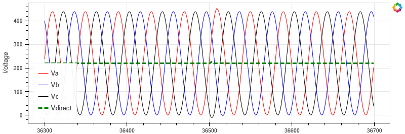
5.1.10.5. RMS Voltage analysis#

A common task for electrical waveform analysis is to convert the three-phase AC voltage into the DC-equivalent using RMS. Quasar provides native support for this using the quadratic_mean function.

The direct current is represented as green in the chart below:

q = """
SELECT
    $timestamp,
    avg(Va) as Va,
    avg(Vb) as Vb,
    avg(Vc) as Vc,
    (quadratic_mean(Va) + quadratic_mean(Vb) + quadratic_mean(Vc)) / 3 AS Vdirect

FROM \"{}\"
IN RANGE (2021-09-12T12:00:00, +1h)
WHERE payload_id = {}
GROUP BY 10ms
""".format(sensor_id, payload_id)
df = qdbpd.query(conn, q)
_ = plot_waveform(df[['Va', 'Vb', 'Vc', 'Vdirect']], highlight='Vdirect')

5.1.10.6. Surge detection#

We can detect surges by detecting variance in the amplitude of each of the currents.

For each cycle, we can calculate the amplitude by comparing the min and the max. As the amplitudes should be constant, it allows us to detect surges.

q = """
SELECT
    $timestamp,
    max(Va) - min(Va) AS amp_a,
    max(Vb) - min(Vb) AS amp_b,
    max(Vc) - min(Vc) AS amp_c

FROM \"{}\"
IN RANGE (2021-09-12T12:00:00, +1h)
WHERE payload_id = {}
GROUP BY 500ms
""".format(sensor_id, payload_id)
df = qdbpd.query(conn, q)

_ = plot_waveform(df[['amp_a', 'amp_b', 'amp_c']], aspect_ratio=3)

5.1.11. Conclusion#

And with this we have finished this waveform ingestion tutorial.

In this guide we have covered:

How to model waveform data in Quasar;

How to convert raw waveform payloads into the correct shape;

Ingesting this data into Quasar using the Pandas integration;

How to query and resample this data;

How to calculate the RMS of a waveform to convert alternating current to direct current;

How to use amplitude detection to detect outliers.